

Imagine: A newly acquired dataset is being prepared for use as a vector database to retrieve information, create recommendation systems, be used for threat detection or similarity-based alert triage. During integration, however, operational challenges surface. Platform constraints prevent full-scale ingestion, prompting an arbitrary reduction in the size of the dataset. As a result, performance degrades significantly. The dataset and dimensionality are still large enough that the indexing methods the vector databases use are making points unreachable. What was intended to be a high-value feature for detection or enrichment instead becomes a bottleneck — difficult to rationalize internally and unreliable from a customer-facing perspective.
In cybersecurity, this problem is all too common, and a lot of it has to do with the nature of the data. For example, traditional malware defense mechanisms rely on algorithms to take a file and return a fixed-length, seemingly random combination of letters and numbers — commonly referred to as a hash — that uniquely identifies the file. As it’s meant to be a unique identifier, even changing a single character will generate a completely different hash. A list of known malicious file hashes can be compiled and integrated into a blocklist, enabling endpoint protection systems to immediately prevent execution if such a file is encountered on a customer’s machine.
However, adversaries can easily circumvent this defense mechanism. By modifying a single byte within the file, the resulting hash becomes entirely different — rendering the new variant unrecognizable to systems relying solely on static hash-based detection. Even minor alterations lead to significant changes in the hash output, as demonstrated below, effectively evading traditional signature-based security controls.

If a threat actor can generate a large number of malware files simply by altering the hash, cybersecurity tools and the experts tasked with monitoring them will find themselves trapped in an endless game of whack-a-mole. This leads to bloated datasets that are hard to fit into traditional vector databases, and that’s before considering the similar, near-duplication that can exist on the benign side of making minor edits to safe files.
Solving the Challenge of Scaling Vector Databases
Faced with this challenge, it’s understandable some security teams simply decide, “Maybe we don’t need all this data.” Rather than processing the entire dataset, a random sampling approach is often applied to reduce the volume to a manageable subset. To analyze the distribution, each file’s content can be encoded into a two-dimensional vector representation using an appropriate embedding or feature extraction technique. The red regions below indicate high-density clusters — typically corresponding to heavily replicated or polymorphic files often associated with evasive malware. In contrast, black regions represent sparse, low-density areas, likely containing benign or non-obfuscated files that were not crafted with evasion techniques in mind.
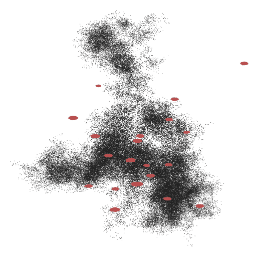
If the red regions constitute 90% of the dataset, then uniform random sampling will disproportionately select samples from these areas. This leads to overrepresentation of redundant or evasive file variants and underrepresentation of sparse, potentially more diverse or novel files.
To ensure a more balanced and representative subset, a more sophisticated sampling strategy is required.
The Drawbacks of Clustering
Clustering may appear to be a natural approach — partition the dataset into clusters and design systems or models around those groupings. However, practical implementation introduces significant challenges, particularly in how clustering algorithms compute and optimize pairwise distance functions.
A key concern is computational complexity. Many clustering methods require evaluating distances between all sample pairs, which can quickly become computationally expensive. For context, Big O notation describes algorithmic complexity: constant time O(1), linear time O(n), quadratic time O(n²), and beyond. In clustering scenarios, especially with high-dimensional data or large datasets, complexity often reaches O(n²), significantly increasing processing time and resource consumption. Keeping this computational overhead low is essential to ensure scalability and operational efficiency.
- Brute-Force Search (Exhaustive k-NN):
- Given a dataset of N vectors of dimension D, brute-force search requires computing distances for all N vectors.
- A typical distance metric such as Euclidean distance has a complexity of O(D) per computation, leading to an overall search complexity of O(ND) per query.
- For a billion-scale dataset (N = 109), this approach becomes prohibitively expensive.
- Approximate Nearest Neighbor (ANN) Algorithms:
- ANN methods like HNSW (Hierarchical Navigable Small World) or FAISS-based IVF (Inverted File Index) reduce complexity to O(logN) or even sublogarithmic in some cases.
- However, they still rely on a large number of pairwise comparisons and require high memory overhead.
- ANN-based methods also suffer from accuracy trade-offs and struggle with dynamic updates.
The Power of Novel Partitioning Methodologies
To address the challenges and shortcomings of clustering, a novel approach is required. Leveraging patented algorithms, the objective is to partition the dataset using a method that operates in linear time complexity, O(n). This allows for scalable processing while preserving representational diversity across the dataset, enabling efficient downstream tasks such as detecting threats or anomalies, as well as behavior modeling” without overwhelming system resources.
With this approach, it is possible to find a file to represent each partition, and select the desired number of partitions to get a dataset that will not overly weight itself to highly replicated files.
How To Utilize Novel Partitioning
The size of the vector database can be tailored by selecting a desired number of partitions and identifying a representative point within each partition that best captures the characteristics of the data in that segment.
The visualization below illustrates this process: beginning with a full dataset, it is partitioned into segments, and a representative point is chosen from each. These representative points form the basis of a primary structure referred to here as the Main Vector Database. This method significantly reduces the number of vectors required while preserving meaningful coverage of the overall data distribution. In cybersecurity applications, attributes such as threat category, malware family, or behavioral label associated with the nearest representative points can be used to infer characteristics of incoming queries.

For scenarios requiring full data coverage—where any original data point must remain accessible—a hierarchical cascade can be implemented. Each partition from the Main Vector Database is linked to a corresponding Partitioned Vector Database, containing similar vectors within that partition. At query time, the system first identifies the closest partitions using the Main Vector Database, then searches within the associated Partitioned Vector Databases to retrieve the most relevant matches. For example, retrieving the top five nearest representative vectors and performing a refined search within those corresponding partitions ensures both scalability and high-resolution retrieval.

How To Update a Single Main Vector or Cascading Vector Database
Single Main Vector Database:
- Take a sample of the existing representative points within the vector database and profile their distances to their nearest neighbors.
- Select the median of these distances to use as a threshold. Use lower or higher quartiles depending on the desirable tradeoff between representation versus database size.
- For any new point that we pass to the vector database, we will check if its distance to the closest point is within the threshold distance.
- If the point is outside the threshold distance, it is added it to the vector database.
Note that further considerations can be made to include datapoints within the threshold distance, for example, if they have opposing labels.
Cascading Vector Database:
- Find the partition that a new point belongs to in the Main Vector Database.
- Find the associated Partitioned Vector Database that houses points for the partition and add the point to that database.
- If desired, see if the central representative point changes with this update in the Partitioned Vector Database, replace it in the Main Vector Database.
How This Aids Efficiency
To demonstrate the value of this approach, consider methods for trying to find the nearest neighbors from a dataset size N where the vectors have dimensionality D. For algorithms that produce clusters, denote the number of clusters as K, where K << N.
| Method | Clustering Complexity | Querying Complexity | Update Complexity | Comment |
| Brute-Force Exhaustive KNN | 𝒪(1) No clustering is required, so the complexity is constant |
𝒪(ND) The querying time is prohibitive as, for a single record, it scales with the size of a database and the dimensionality |
𝒪(1) The only update cost is to add the new record to the database where the rest are stored |
Here the querying complexity 𝒪(ND) is prohibitive on very large datasets, rendering this approach unworkable in such cases |
| K-means or hierarchical methods | 𝒪(NK) Creating the clusters to aid based on the number of initial datapoints and how many clusters are desired to be created |
𝒪(KD) Reduce this complexity significantly from a factor of N to K by querying clusters instead of all points |
𝒪(K)
|
Here the clustering complexity 𝒪(NK) can be prohibitive, for example on datasets measured in billions, and desired clusters as representative points in millions, which can still explode to 10⁹ × 10⁶ = 10¹⁵ |
| Novel Partitioning | 𝒪(N) → 𝒪(3N) The clustering complexity is now only proportional to the size of the dataset, and there is an element of the algorithm that can be repeated (for example, three times) with modification to mitigate tradeoffs to efficacy |
𝒪(KD) The querying complexity remains the same as other approaches for exact matches, but can be 𝒪(K²) → 𝒪(3K) for approximate results |
𝒪(K)
|
The most expensive part will still be building the clusters, but scaling only with the size of the dataset makes this much easier to scale to massive datasets, retaining the same querying complexity (or better) of other methods |
Key Takeaways
Challenges:
- Too many files to reasonably fit into a vector database
- No good way to sample the data that could scale to large datasets
Using the methods outlined above, it is possible to accomplish the following:
- Scalability: Support billion-scale datasets while keeping query times low
- Storage: Require only fractional storage compared to traditional vector databases
- Query Performance: Directly impact latency-sensitive applications like real-time AI search or cybersecurity threat detection
Conclusion
A pairwise, distance-based approach to vector search is costly and scales poorly for very large datasets. By leveraging a novel, representative partitioning approach, it is possible to reduce redundant computations, improve query speed, and lower storage costs. This method is particularly valuable for large-scale AI applications, search engines, and the thigh-dimensional and high-prevalence of near-duplication found in cybersecurity datasets.